tds2el_analyse_maxima: prealignment and refinement of geometry¶

the following documentation has been generated automatically from the docstrings found in the source code.

The aim of tds2el_analyse_maxima_fourier is to do an alignement of the sample

and a refinement of a selectable set of alignement and geometry parameters. In the first phase it can be runned to just convert maxima positions to reciprocal space points. This is done with option

transform_only  = 1 # or True

It will the generate a three columns file q3d.txt containing reciprocal space points.

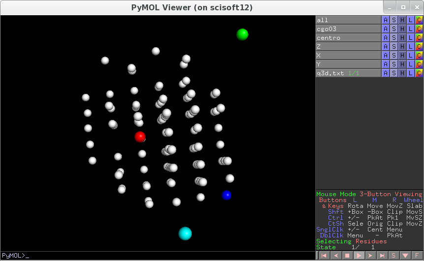
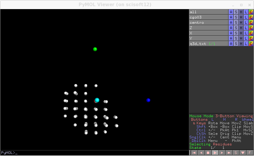
These points can be visualised in 3D graphics using tds2el_rendering. The idea is that when the initial parameters are not too bad and the conventions are not wrong, then the points should be regularly placed in 3D space. Then and only then transform_only can be set to 0, and refinement can start, first by aligning the sample and finding approximate lattice parameters, Then by global optimisation.

tds2el_analyse_maxima_fourier is always runned with two arguments
tds2el_analyse_maxima_fourier  input_file
An example of input file is given below. As a first step you can simply convert the maxima prositions, that you have extracted with tds2el_extract_maxima, to 3d points in reciprocal space. To do this you need to have a rough idea of the geometry pdf and to set the option transform_only = 1.
Supposing that you have done a first run with transform_only=1 , then a three-columns file q3d.txt has been produced with reciprocal space positions. You can have a look at how regular it is. If points are regularly placed, then we can proceed to the further steps which consists in aligning the sample and fine refinement of the geometry. To visualise the maxima in reciprocal space
tds2el_rendering q3d.txt
Example of input file to verify preliminary alignement (transform_only=1) and then to align the sample axis (transform_only=0). Geometry is described here. Multiple solutions exists:as an example here you would get a good alignement with orientation_codes=2, instead of 0, if you change sign to kappa and omega(for this particular geometry).
#########################################
### Really important parameters
## to be set to discover what the geometry conventions
## really are

maxima_file = "selectedpeaks2.p"

orientation_codes=0  # 8 possibilities look at analyse_maxima_fourier.py
theta =  19.0
theta_offset = 0.0

alpha = 50.0
beta = 0.0
angular_step = +0.1

det_origin_Y = 548.0 
det_origin_X = 513.0-20

dist = 244.467
pixel_size = 0.172
kappa = 60.0
omega = -20.3

transform_only  = 1

# lmbda is not so important in the desperate phase. It just expand the size of the lattice
lmbda = 0.98

#####################################################
### Other parameters that are generally small or that can
##  be refined later like r1,r2,r3
beam_tilt_angle = 0.48067
d1 = -0.19731
d2 = -0.37025
omega_offset =  0
start_phi = 0
r1 =  0
r2 = 0
r3 =  0
ftol = 1.0e-7
AA = 0
BB = 0
CC = 0
aAA = 90
aBB = 90
aCC = 90

variations =  {
}
Fourier alignement : To get the alignement of the sample set transform_only=0. When r1,r2,r3 are all equal to zero, this triggers an automatic finding of the cristallography axis by a study of the Fourier transform of the peak distribution. In the above example aAA,aBB,aCC are given. This constraints the found axis to have cosinus which are at no more than a 0.05 distance from the cosinus of aAA,aBB,aCC. If one of these is None, no particular constraint is applied on that cosinus. The axis are searched in the order a,b,c from the shortest to the longest.
in some difficult cases you may use lim_aa variable which must contain lower and upper limit for AA ( Angstroems units)
lim_aa = [4.0,4.4]
which helps finding the proper first axis.
By running tds2el_analyse_maxima_fourier input_file you get an estimation of the alignement
scisoft12> tds2el_analyse_maxima_fourier_v1  ana2.par
MPI LOADED , nprocs =  1
tds2el_v1.analyse_maxima_fourier
Image Dimension : 1043 981
 FMOD  15
 FMOD  19
 FMOD  23
#############
ESTIMATION by FOURIER 
AA=5.342002e+00
BB=6.766536e+00
CC=8.191069e+00
aAA=9.036321e+01
aBB=9.014279e+01
aCC=8.920714e+01
r3=-1.630977e+02
r2=3.897638e+01
r1=-9.677916e+01 
 ############################ 
 processo  0  aspetta 
In reality you get several possible choices. You may have several choice first because of the symmetry operation, second because fro some lattices, like Calcite, the same distribution of Bragg peaks can be fitted with almost as good precision with a wrong set of axis having very close AA,BB,CC and angles but the wrong orientation. When several choices are possible they are ranked according to the suggestion given by the inputted AA,BB,CC, the choice which is closest to the inputted combination of AA,BB,CC is printed last, so that it is the most easily visible on the screen. Now you can insert these estimation in the input file, and see how well it is aligned now by resetting transform_only=1, with subsequent regeneration of q3d.txt and rendering
You can update the input file with these parameters, then to do a further optimisation, you can express the search range around some selected variables
variations =  {
    "r1": minimiser.Variable(0.0,-2,2),
    "r2": minimiser.Variable(0,-6,10),
    "r3": minimiser.Variable(0.0,-2,2) ,
    "AA": minimiser.Variable(0.0,-0.1,0.1),
    "BB": minimiser.Variable(0.0,-0.1,0.1),
    "CC": minimiser.Variable(0.0,-0.1,0.2),
    "aAA": minimiser.Variable(0.0,-0.1,0.1),
    "aBB": minimiser.Variable(0.0,-0.1,0.1),
    "aCC": minimiser.Variable(0.0,-0.1,0.2),
    "omega": minimiser.Variable(0.0,-2.0,2.),
    "alpha": minimiser.Variable(0.0,-2.0*0,6.0*0),
    "beta": minimiser.Variable(0.0,-.5*0,.5*0),
    "kappa": minimiser.Variable(0.0,-2.0,10.0) ,
    "d1": minimiser.Variable(0.0,-0.0,0.0),
    "d2": minimiser.Variable(0.0,-0.0,0.0),
    "det_origin_X": minimiser.Variable(0.0,-20,20),
    "det_origin_Y": minimiser.Variable(0.0,-20,20),
    "dist": minimiser.Variable(0.0,-10,10)                  
}
these specify the variations which are added to the nominal values. A variable that is not appearing here is fixed. The syntax is minimiser.Variable(initial_value,min,max). if min and max are equal. The variable is fixed. The used algorithm is simplex descent, which is slow but roboust. The stop is determined by the ftol parameter. During the fit an output is produced at each step with the following form
----------------------------------------------------------------------------------------------------
THESE ARE THE MAXIMUM DEVIATION FROM INTEGER FOR EACH PEAK POSITION
[ 0.00769985  0.00874746  0.0103178   0.01073825  0.01460457  0.01573443
  0.01678818  0.01696467  0.01738405  0.0190767   0.01931381  0.02025402
  0.02047992  0.02066052  0.02079439  0.02093673  0.02123821  0.0218755
  0.02206755  0.02210927  0.02229428  0.02239919  0.02248192  0.0225352
  0.02289104  0.02290201  0.02321625  0.02379918  0.02390862  0.0244956
  0.02491748  0.0251143   0.02519226  0.02532196  0.02573431  0.02581072
  0.02606213  0.02613378  0.02687216  0.02693677  0.02699292  0.02735329
  0.02740729  0.02866364  0.02887559  0.02986479  0.03001773  0.03003705
  0.03034055  0.03042722  0.03121853  0.03122759  0.03131694  0.0313735
  0.03142095  0.03175396  0.03199106  0.03258067  0.03260487  0.03271961
  0.0332849   0.03333455  0.03341007  0.03370857  0.0339517   0.03398085
  0.03427243  0.03504014  0.03567719  0.03595769  0.03609461  0.03629518
  0.03699565  0.03701109  0.037045    0.03711748  0.03732347  0.03821397
  0.03824425  0.03832698  0.03909755  0.03949523  0.04051018  0.04076242
  0.04114318  0.04152346  0.04158688  0.04177046  0.04212689  0.04253507
  0.04272914  0.0432117   0.04632831  0.04675317  0.04820037  0.05184102
  0.0528053   0.05769324  0.05784869  0.05879927  0.05955482  0.06063747
  0.06166363  0.06746936]
 ERROR  0.160689
 ----------------- obtained with variables here below ----------------------
AA  =  5.29437816027
aCC  =  90.0475179112
aBB  =  90.0377539549
aAA  =  89.9699951653
r1  =  -97.0917210501
r2  =  37.4926288928
r3  =  -164.837866817
CC  =  8.49977434955
kappa  =  60.1505399461
BB  =  6.74705222684
d2  =  0.419158100662
beta  =  0.0
det_origin_X  =  506.027292059
det_origin_Y  =  527.678671914
alpha  =  50.0
omega  =  -18.9479007388
dist  =  241.047652156
d1  =  -0.49890822079
if a variable is hitting against one of the border a message is produced so that you can change the search span. The list of numbers is the maximum deviation, for each spot, from the nearest integer for hkl coordinates.

The refined alignement can be visualised again .. image:: pymol_refined_alignement.png

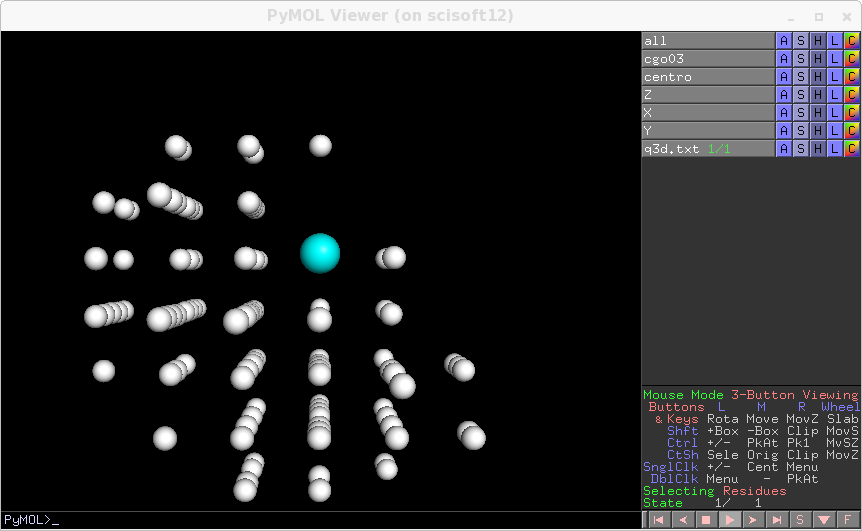
Which is not so bad. Still the deviations from integer hkl are not so small and for a good fit of elastic constants we need to do much better. The discrepancy may come from several effect.

Errors in the peak position detection. This might happen typically if the crystal is big so that the spot is large. or because there is not enough resolution. In this case the subsequent step will consist in fitting the diffused scattering, optimising at the same time the elastic constants and few selected variable of the geometry like r1,r2,r3, kappa, omega, AA,BB,CC. The advantage of this procedure is that the poistion information is distributed in the global envelop of each spot that we can fit globally, and we have many peaks but few geometry parameters.

The sample is very thin, so that the spot are well defined but there may be some mechanical instability, due to the thin sructure, and also x-ray radiation could develop some stress with accompanying deformation. In this case the Bragg spot is very sharp and we can take its position as the center of the spot.

tds2el_analyse_maxima: prealignment and refinement of geometry¶

Previous topic

Next topic

This Page