Introduction to iterative methods
Iterative methods for tomographic reconstruction
The formalism
Instead of performing a one-step, non-parametric reconstruction, iterative methods deals with tomographic reconstruction as an inverse problem :
Where \(P\) is the projection operator (which transforms a volume into a sinogram), \(d\) the acquired data and \(x\) the volume to recover. The associated optimization problem is often :
where \(g(x)\) is some regularization reflecting a prior information on the volume. When \(g = 0\), the problem (1) amounts to a simple least-squares problem. Well-known corresponding optimization algorithms are ART, SIRT and CG-LS.
The need for regularization
When \(g = 0\) in problem (1), the solution is very sensitive to noise. As a practical consequence, in algorithms like SIRT, the number of iterations have to be chosen carefully : if there are too many iterations, the noise is lileky to be overrepresented in the solution.
- Choosing a regularization term \(g \neq 0\) has some advantages :
It brings some stability in the reconstruction process
\(g(x)\) can be designed to include some prior knowledge on the volume. For example, for piecewise-constant volumes (well-separated phases), the Total Variation \(g(x) = \lambda \norm{\nabla x}_1\)
- is an adapted prior.
Some priors are adapted to reconstruct from highly limited data. This is the case for Total Variation.
The optimization problem (1) often becomes non-smooth depending on the choice of \(g(x)\). Hence, dedicated algorithms have to be used.
Using iterative techniques in PyHST2
Please note that these algorithms are implemented to run on GPU, so you need to run PyHST with a GPU to use them !
PyHST2 implements some well-known algorithms (FISTA, Chambolle-Pock), and custom algorithms (Conjugate subgradient) as well.
The reconstruction steps are specified with a parameter file, in the format KEY = VALUE.
The key enabling iterative techniques is ITERATIVE_CORRECTIONS, which has to be set to a non-zero value.
The main relevant parameters are the following :
ITERATIVE_CORRECTIONS = 100     # 100 Iterations
DENOISING_TYPE = 1              # Regularization type
OPTIM_ALGORITHM = 1             # Optimization algorithm to use
BETA_TV = 1.0                   # Weight of regularization
There are additional parameters depending on the regularization type, and performance-tuning parameters.
- Currently, 3 regularizations are implemented in PyHST2 :
Total Variation (TV)
Dictionary Learning (DL)
Wavelets
Each of these regularizations (DENOISING_TYPE) have one or more available optimization algorithms (OPTIM_ALGORITHM) to solve them.

Optimization algorithms available depending on the regularization type
Total Variation regularization
In this case, \(g(x) = \lambda \norm{\nabla x}_1\) : the regularization promotes the sparsity in the gradient domain, i.e promotes piecewise-constant images.
This is the simplest and the fastest method, recommended for simple objects.
The corresponding parameters are the following :
DENOISING_TYPE = 1  # Total Variation
OPTIM_ALGORITHM = 3 # 1 for FISTA, 3 for Chambolle-Pock
BETA_TV = 1.0       # Weight of regularization
The Chambolle-Pock algorithm (OPTIM_ALGORITHM = 3) is recommended for Total Variation minimization.
More details are given in the tutorial dedicated on TV regularization.
Dictionary Learning regularization
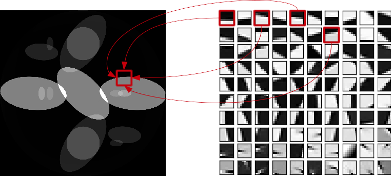
In this case, \(g(x) = \lambda \norm{D x}_1\) where \(D\) is a dictionary transform, mapping a slice \(x\) to a set of coefficients \(w\) in the dictionary basis. This regularization promotes the sparsity in the dictionary domain.

Principle of dictionary-based reconstruction. Every part of the reconstructed image (left) is a linear combination of the dictionary patches (right). The coefficients are found with an optimization procedure.
If the dictionary is learnt on a high quality volume similar to the volume to be reconstructed, this method will be especially efficient. In practice, this method is very robust with respect to the dictionary : the same dictionary can be used to reconstruct a variety of volumes.
The optimization problem can be put in the form
where \(D^*\) is the operator reconstructing a slice from its set of coefficients. A function \(h(w)\) tunes the overlapping when tiling the slice with the dictionary patches. Overlapping patches yield significantly better reconstruction quality, since it avoids the discontinuities arising from the patches tiling.
The relevant parameters for Dictionary-based reconstruction are the following :
DENOISING_TYPE = 4          # Dictionary Learning
OPTIM_ALGORITHM = 1         # 1 for FISTA, 5 for Conjugate sub-gradient
PATCHES_FILE = 'patches.h5' # Location of the dictionary (HDF5 file)
STEPFORPATCHES = 4          # patches step when tiling the image
BETA_TV = 1.0               # Weight of regularization
WEIGTH_OVERLAP = 1.0        # Weight of the overlapping
Here BETA_TV corresponds to \(\lambda\) and WEIGHT_OVERLAP corresponds to \(\rho\) in (2).
Usually, the patches file contains \(8 \times 8\) patches, so STEPFORPATCHES = 4 yields a \(\frac{1}{2}\) overlapping.
This value is seldom changed.
For DL reconstruction, two optimization algorithms are available : FISTA and Conjugate sub-gradient. The latter converges much faster, but is more memory-consuming.
More details are given in the tutorial dedicated on DL regularization.
Wavelets regularization
Total Variation is fast, but promotes piecewise-constant images. On the other hand, Dictionary-Learning is adapted for all volumes, but theoretically requires a dictionary of a good-quality volume. The Wavelets reconstruction was designed to overcome both of these limitations. It is adapted for most practical volumes without requiring a dictionary, and it is reasonably fast.
DENOISING_TYPE = 8  # Wavelets regularization
OPTIM_ALGORITHM = 1 # Only FISTA is available for wavelets
BETA_TV = 1.0       # Weight of regularization
W_LEVELS = 8        # Number of Wavelets decompositions
The parameter W_LEVELS specifies the number of decomposition levels performed by the wavelet transform at each step.
The higher value, the more accurate will be the reconstruction ; it may be a bit slower. The maximum decomposition level is \(\log_2 \left( \frac{N}{K}\right)\) where \(K\) is the kernel size (2 for the Haar wavelet) ; for example 10 for a \(2048 \times 2048\) slice.
More details are given in the tutorial dedicated on Wavelets regularization