Multi Paganin Tutorial
For this tutorial we are going to use the material provided with the non regression tests. Therefore we assume that you have installed and runned all the nonregression tests as described here Non Regression Tests.
In particular we will use the multipaganin nonregression test. Supposing that you have runned the nonregression tests, and that as output target you have chosed
outputprefix="/tmp/tests"
you can now go to the output directory
/tmp/tests/MULTIPAGANIN/TESTS/volume
and there you will find several input files and one output
>ls -tl
-rw-r--r--  Oct  2 17:08 vol.vol.info
-rw-r--r--  Oct  2 17:08 vol.vol
-rw-r--r--  Oct  2 17:08 multipaganin_input.par_5.par
-rw-r--r--  Oct  2 17:03 multipaganin_input.par_4.par
-rw-r--r--  Oct  2 17:00 multipaganin_input.par_2.par
-rw-r--r--  Oct  2 16:55 multipaganin_input.par_0.par
-rw-r--r--  Oct  2 16:55 machinefile
-rwxr-xr-x  Oct  2 16:55 input.par
The principal file is input.par. All the other files are automatically generated and runned by the different steps. The provided input.par file is already configured in order to perform all the steps, and with the good parameters.
We are now proceding from scratch, pretending we dont know yet the good parameters.
First do a copy of the input file
cp input.par myinput.par
Then edit myinput.par and remove these lines and all the lines below
# Multi_paganin
# 2nd delta over beta ratio for multi Paganin phase retrieval = 150.00
MULTI_PAGANIN_PARS={}
.......
.......
and all the lines below
OK. Now your myinput.par is a simple file which normally does a Paganin reconstruction with
PAGANIN_Lmicron = 293.497325
which is adapted for the flesh regions but not for the bones. test it by reconstructing
PyHST2_2017c myinput.par scisoft12,0
If you are on scisoft12 and using GPU 0. Change the host name for your case. If you dont have a GPU
PyHST2_2017c myinput.par
should work all the same but be much slower : this example is in conical geometry and the conical projector/backprojector are much slower withour GPU. Things should be better if you rework the tutorial on a parallel geometry case. Mind however that with multi-paganin you cannot reduce too much the number of slices ( which could be an idea to speed up things). This because the Paganin kernel is a 2D kernel wich acts on projections, so you must consider a certain slab of slices so that the ones in the middle are correctly computed when in the Multi_Paganin procedure back-projection and projections are alternated during the different steps.
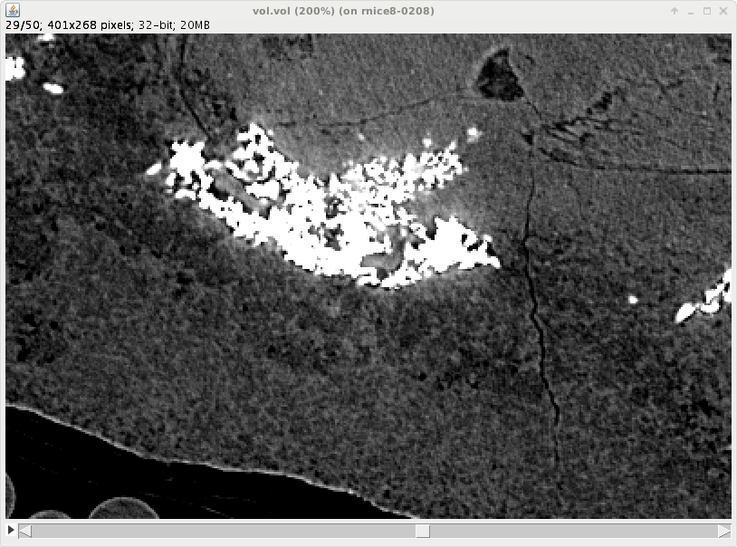
If you have now reconstructed with the simplidief myinput.par you can now open the reconstructed volume and visualise the effects of not using the multi-Paganin reconstruction
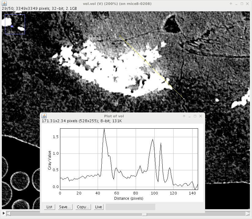
You can see that around the bone highly absorption feature, the signal is leaking. This happens because the PAGANIN_Lmicron is tuned for the flesh optical constants.
Now we are going to work step-by-step the application of the multi-Paganin method to this case. Add at the end of myinput.par
MULTI_PAGANIN_PARS={}
MULTI_PAGANIN_PARS["BONE_Lmicron"]= 131.255994
MULTI_PAGANIN_PARS["THRESHOLD"]= 1.2345
MULTI_PAGANIN_PARS["DILATE"]= 2
MULTI_PAGANIN_PARS["MEDIANR"]= 4
This would be all if we were sure of all the parameters, but we have put here the fantasy parameter
MULTI_PAGANIN_PARS["THRESHOLD"]= 1.2345
to underline that we dont know yet the threshold for the bone-flesh segmentation. Therefore we perform here only one step of the seven steps composing the method, this in enforced by setting this optional parameter
MULTI_PAGANIN_PARS["STEPS"]= [1,0,0,0,0,0,0]
which by default is a list of seven numbers 1. A number 1, at position m in the list, means perform mth step and a 0 means dont. Therefore we are performing now only the first step. \(BoneMask*(AbsVol-AveragerOperator(BoneMask,AbsVol) )\) The steps are (look only at the first one for the moment) :
STEP 1) generates a volume (call it BoneVol) reconstructed with the Paganin parameter adapted for bones.
STEP 2) From this volume generates the bone mask (call it BoneMask) volume according to the threshold, the radius for the median filter window and the dilatation.
STEP 3) generates the absorption reconstruction (call it AbsVol) from raw data ( no Paganin filtering)
STEP 4) generates by subtractions and multiplications a new volume which contains the bone contribution that we will subsequently projects away from the raw data. This volume ( call it CorrBoneVol) is obtained as \(BoneMask*(AbsVol-AveragerOperator(BoneMask,AbsVol) )\). The symbol AverageOperator stands for a routine which propagates inside the BoneMask region the values that are external to the mask. In other words the values of AbsVol at pixels close to the thresholding surface, the one obtained by thresholding and dilatation.
STEP 5) generates a set of projections from CorrBoneVol.
STEP 6) generates NoBoneVol from the original data but with the projections from step 5 subtracted from the raw radiographies before applying Paganin.
STEP 7) Produces the final result merging together NoBoneVol and BoneVol according to BoneMask.
Our aim in this tutorial is looking at what is going on at the different steps. PyHST2 proceeds by creating temporary files which are canceled at the end of the run. These files are written into a scratch directory which defaults to /tmp (you can change it, look here Multi Paganin). Alternatively you can choose location for them with the following instraction, this way they will remain at the selected location and will not be canceled
MULTI_PAGANIN_PARS["PAGBONE_FILE"] =      "/tmp/multipag_bone.vol"             # BoneVol
MULTI_PAGANIN_PARS["MASKBONE_FILE"] =     "/tmp/multipag_mask.vol"             # BoneMask
MULTI_PAGANIN_PARS["ABSBONE_FILE"] =      "/tmp/multipag_abs.vol"              # AbsVol
MULTI_PAGANIN_PARS["CORRBONE_FILE"] =     "/tmp/multipag_corr.vol"             # CorrBoneVol
MULTI_PAGANIN_PARS["CORRPROJSPATTERN"] =  "/tmp/tmppnohHx.vol/proj_%05d.edf"   # the pattern used to write the projections of CorrBoneVol
MULTI_PAGANIN_PARS["CORRECTEDVOL_FILE"] = "/tmp/multipag_soft.vol"             # NoBoneVol
running myinput.par we obtain the reconstruction /tmp/multipag_bone.vol
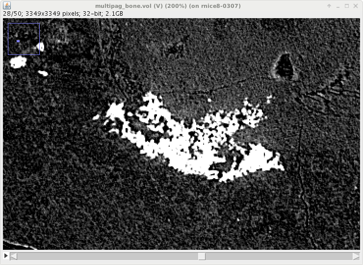
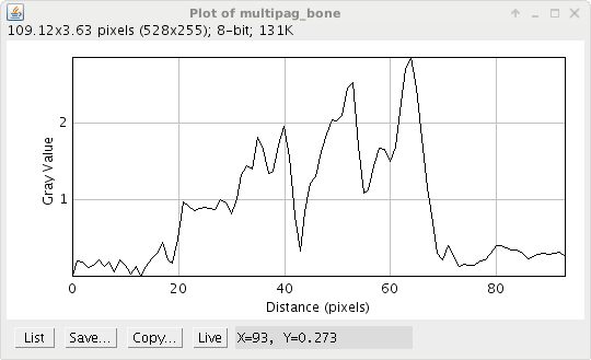
where the bone signal has less spilling over the neighbouring regions. Looking at the bone profile we can select an appropriate threshold, here 0.370
MULTI_PAGANIN_PARS["THRESHOLD"]= 0.370
The following step is the segmentation. This operation depends on the parameters THRESHOLD and DILATE. If you want to optimise them you can activate just the steps 2 /tmp/multipag_mask.vol. Then you can see the effect of the parameters on the mask shape. We proceed here with the provided data which are not too bad and activate all the steps :
either set to 0 the first which is already done an activate the six remaining steps.
or more simply remove the instruction MULTI_PAGANIN_PARS[“STEPS”]= …. You will perform by default all the steps
Once you have performed all the steps, you will find the intermediated results in the selected location. We are going to look at these results to understand how the code works.
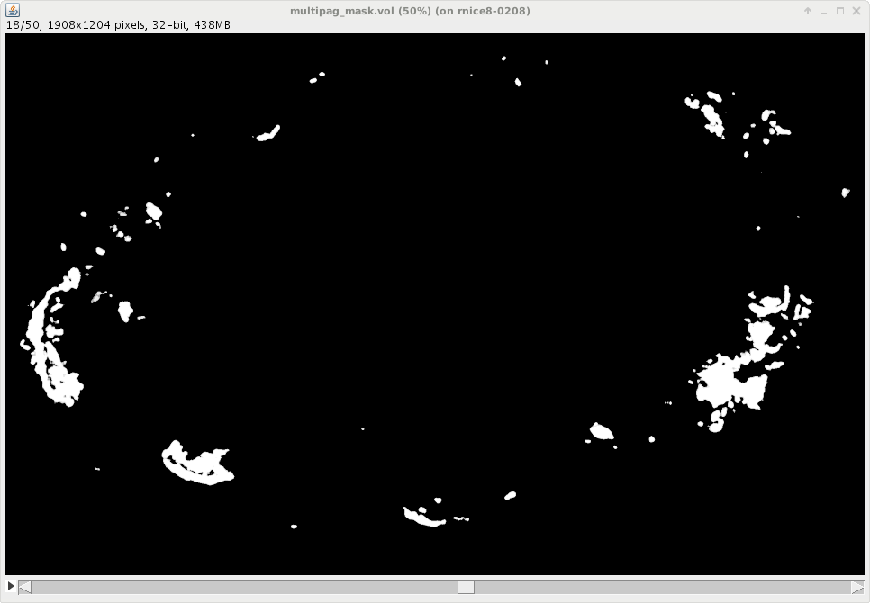
Step 2 consists in generating the bone mask (call it BoneMask) volume according to the threshold, the radius for the median filter window and the dilatation. How it works : a median filter is applied on the volume from step 1(Paganin parameter for the bone) and then thresholding. The obtained mask is further dilated. Here the result :
At step 3 we reconstruct the volume with no Paganin filter at all :
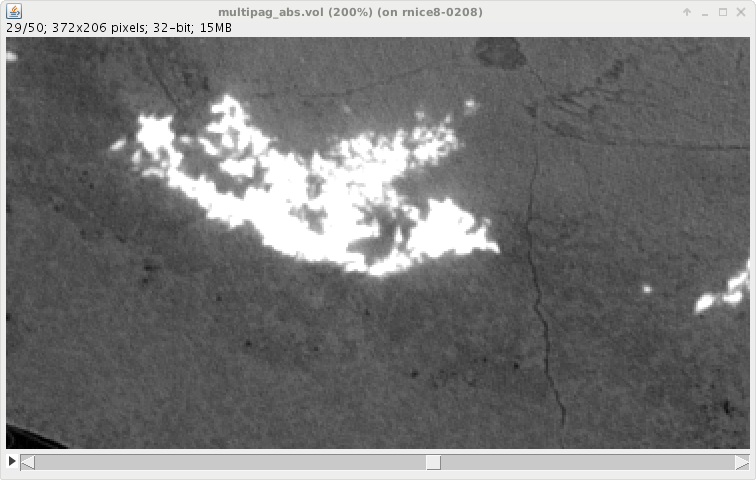
- The obtained volume is more noisy but it is a localised representation of the raw signal :
while in the raw sinogram everything is mixed together
the reconstructed volume, althought inexact due to interference fringes, localises the bone contribution inside the mask region. From this volume we build the correction : it is generated as \(BoneMask*(AbsVol-AveragerOperator(BoneMask,AbsVol) )\). The symbol AverageOperator stands for a routine which propagates inside the BoneMask region the values that are external to the mask. In other words the values of AbsVol at pixels close to the thresholding surface, the one obtained by thresholding and dilatation :
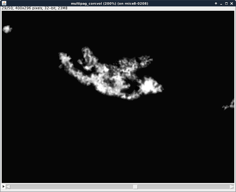
This correction contains the signal from the bone. We wish to remove it from the raw signal, so that we can apply, on the result, the Paganin filter which is appropriate for the flesh. In order to do so at step 4 the correction volume is projected and we obtain a set of projection, this is one :

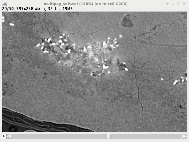
In this example we are working on a tiny slab of 50 slices. The Paganin filter in this example is not very important : it is of the order of hundred microns while a pixel is 45 microns. What is important to know, when the Paganin length is large, (in general this is the case if you are interested in Multi-Paganin) is that the Paganin filter is a 2D convolution applied on the projection, this means that you have good result in the interior of the slab. If your Paganin-filter is large, a good choice is to reconstruct the whole volume rather than just one slice. This will be visible in the bone-less reconstruction. The bone-less reconstruction is performed at step 6) : the volume is reconstructed with the Paganin lenght for the flesh but starting from the cleaned data :
and finally step 7) puts the two components together :
