Getting Calcite constants out of TDS, a worked out example
On the ftp site where this documentation is,
you can find first the input file for peaks extraction
extraction.par
here how it looks
images_prefix             =  "data/Calcite_170K_1_0"

# Let the following images_prefix_alt to None and dont set it ( default None)
# It is used for reviewing with comparison of same position locations
# versus an alternative dataset
#  images_prefix_alt         =  "G19K45/set1_0001p_"
images_postfix        =  ".cbf"

## peaks are searched, having a radius peak_size
#  and with maximum > threshold_abs and > image_max*threshold_rel
threshold_abs=40000
threshold_rel=0.00
peak_size = 2
spot_view_size = 10

# Filtering, OPTIONAL or set it to None for no mask filtering of bad pixels
# filter_file           =  None
filter_file           =  "data/filter.edf"

##  medianize can be 1 or 0 ( True or False)
##  The peak is always searched into a stack
##  of spot_view_size + 1 + spot_view_size slices
##  When the option is activated each slice will be beforehand
##  subtracted with the median of the  slices going from the spot_view_size^th preceeding
##  to the spot_view_size^th following. Spot_view_size should be greaer than peak_size
medianize = 1


## Let this advanced option as it is for now, or dive into the code.
## The rationale here would be that in the first step on works
## locally on spot_view_size + 1 + spot_view_size slices,
##  in the second step one can work globally on the found peaks
globalize = (0,0)

## The file where  found peaks are written
## or, when reviewing, read.
file_maxima = "maxima.p"

### if yes, a graphical window allows for the selection of the mask
### Closing the window will propose to write on newmask.edf
drawmask = False

## Allows to have a simultaneous and animated view of the blobs.
## Animated thumnails.
## They can be selected of deselected. When clicking on the
## thumbnails a larger 3D explorer is charged with
## a (review_size+1+review_size )^3 stack
review = False
review_size = 50
- that you use on the data that you can download(3G!!!) here
calcite.tgz.
You have to create a directory test and you write there extraction.par and you untar there calcite.tgz. This will create the image files in subdirectory data of test.
Do first a peak detection run, that will extract approximate peak positions which will be used for geometry alignement
tds2el_extraction_maxima_vX extraction.par
where vX is the version number (you can set it in __init.py before installation).
This generates file maxima.p as requested. We are going to use these peak positions to align the sample. You can check that all the peaks are meaningful for an alignement by setting review to True and rerun, but we are not discarding any for the moment(if you want you can already view the peaks by setting review to True but dont discard them unless there is a good reason because the alignement of the sample runs better with more peaks)
We are now going to use maxima.p for the alignement.
First we use the file ana0.par.
#########################################
### Really important parameters
## to be set to discover what the geometry conventions
## really are


orientation_codes=7  # 8 possibilities look at analyse_maxima_fourier.py
theta =  0.0
theta_offset = 0.0

alpha = 50.0
beta = 0.0
angular_step = +0.1

det_origin_X = 1242.06
det_origin_Y = 1258.6

dist =  299.987
pixel_size = 0.172
kappa = 0
omega = 90


# lmbda is not so important in the desperate phase. It just expand the size of the lattice
lmbda = 0.6968

#####################################################
### Other parameters that are generally small or that can
##  be refined later like r1,r2,r3
beam_tilt_angle = -0.05118

d1 = 0.04845
d2 = 0.1531

omega_offset =  0
phi = 0


##################################
# AA,BB,CC r1,r2,r3 : we will find them later
############################"
## aAA, aBB, aCC... later


################################################
###### peaks positions are read from this file
maxima_file = "maxima.p"


###########################################################################
## we are going to visualise the spots distribution in reciprocal 3D space
##
transform_only  = 1
In this file we have put a rough knowledge of the experimental geometry and we have not set r1,r2,r3 yet, that must be aligned, and cell parameters neither. The first step is a visual check of the experimental geometry, which is triggered by setting, in ana0.par; transform_only to 1, so that q3d.txt will be generated by the following command:
tds2el_analyse_maxima_fourier_v1 ana0.par
and then visually inspected by
tds2el_rendering_v1 q3.txt
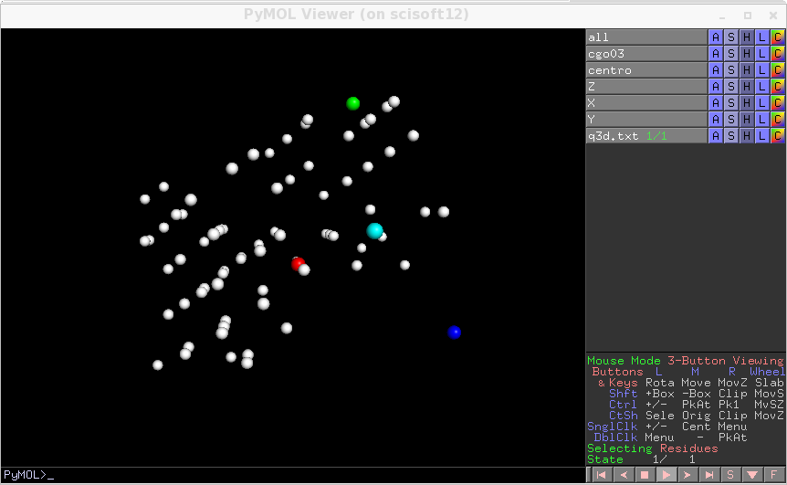
The regular distribution of peaks is a sign that the geometry is correct. If you change ordering_codes ( the orientation of the detector) you may happen to find another choice of the orientation which works correctly, here the alternative would be 5. We do here the procedure with choice 7. Otherwise you can have slightly wrong parameters and still have a usuable prealignement. In this case an error of 10 or more pixels on the detector zero, would not be dramatic and you can use a rough idea of the geometry to bootstrap and refine later the uncertain parameters.
Given that the alignement is not so bad
rerun with this this.
input file . Fourier alignement is now performed, due to r1,r2,r3 set to zero*which triggers the alignement
of the sample. Here how the input file looks like
#########################################
### Really important parameters
## to be set to discover what the geometry conventions
## really are

maxima_file = "maxima.p"

orientation_codes=7  # 8 possibilities look at analyse_maxima_fourier.py
theta =  0.0
theta_offset = 0.0

alpha = 50.0
beta = 0.0
angular_step = +0.1

det_origin_X = 1242.06
det_origin_Y = 1258.6

dist =  299.987
pixel_size = 0.172
kappa = 0
omega = 90

# lmbda is not so important in the desperate phase. It just expand the size of the lattice
lmbda = 0.6968

#####################################################
### Other parameters that are generally small or that can
##  be refined later like r1,r2,r3
beam_tilt_angle = -0.05118

d1 = 0.04845
d2 = 0.1531

omega_offset =  0
phi = 0

##################################
# AA,BB,CC r1,r2,r3 : settint r1,r2,r3 to zero
# triggers Fourier estimation of  r1,r2,r3,AA,BB,CC
# and also aAA,aBB,aCC
############################"
##
r1 =  0
r2 = 0
r3 =  0
AA = 4.98
BB = 4.98
CC = 17.0

## this gives some constraint for the cell angles
aAA = 90
aBB = 90
aCC = 120


################################################
###### peaks positions are read from this file
maxima_file = "maxima.p"
The program stops producing the following estimations
#############
## ESTIMATION by FOURIER
AA=4.899338e+00
BB=4.899338e+00
CC=1.703103e+01
aAA=90.0            ##
aBB=90.0            ##  set by hand
aCC=120.0           ##
r3=-6.352717e+01
r2=6.700895e+01
r1=-1.735652e+02
############################
which is displayed on the screen. In reality several estimations are produced, ranked from the worst to the best according to the distance of the found AA,BB,CC from the values given in input. Copy (choose one if several are available) and paste a set of guessed parameters in the input file so that you get a new file for the next step. You can copy and past this estimation at the end of the ana1.par file, set now transform_only=1 and generate again q3d.txt to see how well it is aligned, remember the definition of GIACOVAZZI where astar is aligned with X axis.
In this run aAA,aBB,aCC where more or less constrained to their initial values and we have set them back to their nominal value. You can free one of them by setting its initial value to None. In all cases the search rejects combination of axis whose 3x3 determinant of their versors is smaller than 0.3(hard-coded parameter). The variable variations is an empty dictionary to signify that the program has to stop after producing the first guess of r1,r2,r3 and axes based on Fourier transform of the peaks distribution.
You can now run a fine retuning of the parameters by resetting transform_only to zero
and adding variation informations for the choosed to-be-optimised variables (see the main documentation for explanations),
we use the file ana2.par,
obtained by adding first the initial guess for r1,r2,r3,AA,BB,CC
and eventually aAA,aBB,aCC, plus the following intervals for
variations at the end of the file,
we have fixed there aAA, aBB, aCC by hand ::
Note that in this optimisation above we have used dipendent AA and BB.
You can set them to vary identically using this mechanism: you use an OrderedDict
which keeps the ordering and, here below, BB which is set to -1
is interpreted to vary with the -1 in relative position, which is AA
variations =  collections.OrderedDict([
    ["r1", minimiser.Variable(0.0,-2,2)            ]    ,
    ["r2", minimiser.Variable(0,-6,10)             ]    ,
    ["r3", minimiser.Variable(0.0,-2,2)            ]     ,
    ["AA", minimiser.Variable(0.0,-0.1,0.1)        ]     ,
    ["BB",  -1   ]  ,
    ["CC", minimiser.Variable(0.0,-0.2,0.2)        ]      ,
  ]
)
## a tolerance. It controls when the fit stops
##
ftol = 1.0e-7
The relative position is taken on the ordered list of independent variables. Therefore for a cubic crystal you should set the variation like this
["AA", minimiser.Variable(0.0,-0.1,0.1)        ]     ,
["BB",  -1   ]  ,
["CC",  -1        ]      ,
because BB is not going in the list of independent variables, then -1 for CC means AA. In some cases it may be useful to add more variables to this dictionary, so that they will be optimised. In our particular case we know already well the geometry and we need to align just the sample.
There is also a more precise retuning of the geometry that we can do at Cij fitting time that we will see later in the documentation.
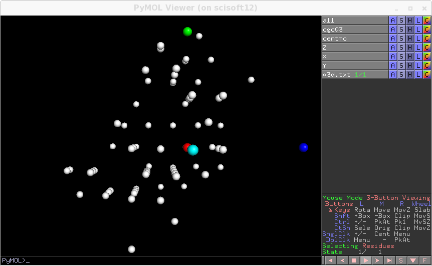
You can now run ana2.par. Now the optimisation is done with simplex descend, which is slow but roboust. You get refined parameters at the end, and at each step they are printed on screen. Reuse them for the next step, of course the first thing to do is to check if they look good, with transform_only=1. You know already how to do, you get this:
At the end of the run a new maxima file tagged_maxima.p is written. Now you can select or discard spots by setting review=True and file_maxima=”tagged_maxima.p” in extraction.par and rerun tds2el_extraction. You generate newpeaks.p
But it is not necessary for now, we will work with the whole set
of peaks.
Now we are finally ready to go to the tds2el core.
We start from the file ana3.par which contains the good geometry.
On this basis we construct tds2el.par :
which is formed adding few parameters to ana3.par (which already contains structural refined
parameters from alignement process):
### To show a list of harvested spots and stop, uncomment line below
## show_hkls = True
##### manual selection, uncomment  line below
### collectSpots  = [[-5, 3, 1], [-5, 3, 4], [-5, 4, 0], [-4, 2, -6], [-4, 2, 0], [-4, 2, 6]]
#  to select spots from peaks file
file_maxima = "newpeaks.p"
### OPTIONS FOR EASY EDITING
DO_HARVESTING = 0
TODO = DO_HARVESTING
if(TODO==DO_HARVESTING):
    threshold = 100000.0
    DeltaQ_max = 0.15
    DeltaQ_min = 0.03
    load_from_file= None
    save_to_file  =  "collection4c.h5"
    DO_ELASTIC=1
and structuring in such a way that you can add new tasks and select them through TODO variable. The threshold parameters is used to filter out all those images with pixel values greater than threshold, while computing for each spot its center which is the weighted average of all points with value exceeding threshold. You can change this behaviour setting variable badradius to greater than zero, for example
badradius=300
to discard not the whole image but a disc of radius 300 around the bad pixels. If badradius==0 then all the image is discarded if only it contains one hot pixel. The harvested file collection4c.h5 will contain these baricenter informations, while the Qs are calculated based on geometry. Then we create the main input file tds2el.inp
conf_file             =  "tds2el.par"
filter_file           =  "data/filter.edf"
images_prefix         =  "data/Calcite_170K_1_0"
ascii_generators      =  "2(110),3(z),1~"
normalisation_file    = "normalisation.txt"
We use the normalisation.txt that we
have created with this script where we rely
on the timestamps to interpolate in the esrf-machine file of the intensities.
NOTE that we had to rely in the script on the files time stamps because all the metadata of one single scan files
are all identical copy-and-paste. This might not be a problem though because for this Calcite example
we are going to retrieve the relative elastic constants which depend mainly
on the TDS shape around each peak, each peak being fitted with an ad-hic factor, and
that a sweep through an hkl spot is relatively fast. Multiple sweep across the
same hkl, we repeat it, are fitted separately with two independent factors.
When you run the harvesting, you can gain some time using mpi for parallel processing
mpirun -n 12 tds2el_v1 tds2el.inp
Then you have a lot of message flowing on the screen, you can check at least than in the lines like the one below, the hkl for the maximum of the image , at least the maximum with big value, are at close-to-integer values
the maximum is 1.15984e+06 [ 0.58050209 0.60439211 -0.23556644] and hkl are [ 0.99992228 3.01368737 -4.00607014] fname data/Calcite_170K_1_0113.cbf i,j (array([2000]), array([248]))
Now we redo a harvesting but a centered one this time, and we write it on collection_centered.h5 using the centering informations contained in collection4c.h5 to shift the spots blobs
DO_CENTERED_HARVESTING = 1
TODO = DO_CENTERED_HARVESTING
if(TODO==DO_CENTERED_HARVESTING):
    centering_file ="collection4c.h5"
    threshold = 100000.0
    DeltaQ_max = 0.15
    DeltaQ_min = 0.03
    load_from_file= None
    save_to_file  =  "collection_centered.h5"
    DO_ELASTIC=1
and rerun the harvesting obtaining collection_centered.h5.
Now do a dry run
DRY_RUN=2
if TODO == DRY_RUN:
    DO_ELASTIC=1
    load_from_file= "collection_centered.h5"
    save_to_file  =  None
    fitSpots = True
    file_maxima = "tagged_maxima.p"
    REPLICA_COLLECTION = 0
Getting the tensor structure
 GET ELASTIC SYMMETRY
1.000000 A11  | 1.000000 A11  | 1.000000 A13  |               | 1.000000 A15  |
              | -2.000000 A66 |               |               |               |
---------------------------------------------------------------------------------------------
1.000000 A11  | 1.000000 A11  | 1.000000 A13  |               | -1.000000 A15 |
-2.000000 A66 |               |               |               |               |
---------------------------------------------------------------------------------------------
1.000000 A13  | 1.000000 A13  | 1.000000 A33  |               |               |
              |               |               |               |               |
---------------------------------------------------------------------------------------------
              |               |               | 1.000000 A44  |               | -1.000000 A15
              |               |               |               |               |
---------------------------------------------------------------------------------------------
1.000000 A15  | -1.000000 A15 |               |               | 1.000000 A44  |
              |               |               |               |               |
---------------------------------------------------------------------------------------------
              |               |               | -1.000000 A15 |               | 1.000000 A66
              |               |               |               |               |
[(0, 0), (1, 1), (2, 2), (3, 3), (4, 4), (5, 5), (0, 1), (0, 2), (0, 3), (0, 4), (0, 5), (1, 2), (1, 3), (1, 4), (1, 5), (2, 3), (2, 4), (2, 5), (3, 4), (3, 5), (4, 5)]
 THE ELASTIC TENSOR VARIABLES ARE
['A11', 'A33', 'A44', 'A66', 'A13', 'A15']
 NOW STOPPING, TO DO TRHE FIT YOU NEED TO SET CGUESS
 processo  0  aspetta
And finally the last step
FIT=3
TODO = FIT
if TODO == FIT :
    DO_ELASTIC=1
    load_from_file= "collection_centered.h5"
    save_to_file  =  None
    fitSpots = True
    file_maxima = "tagged_maxima.p"

    CGUESS={"A11":  [13.7,0 , 400],
            "A13":  [2.37825229066,-400 ,400 ],
            "A15":  [-2.37825229066,-400 ,400 ],
            "A33":  [7.97 ,-400 ,400 ],
            "A44":  [3.42,-400 ,400 ],
            "A66":  [2.37825229066,-400 ,400 ],
    }

    doMinimisation=1
    visSim=1

    testSpot_beta = 0.06
    testSpot_Niter = 80
    testSpot_N = 128
that you launch NOT in parallel because it goes on GPU (or openCL CPU)
tds2el_v1 tds2el.inp
When we run the here provided tds2el.par input file (the three steps DO_HARVESTING, DO_CENTERED_HARVEST, DOFIT) we get at the last iteration
Cd  [  8.77377685  11.94596129   9.13998372  12.02890254  10.69581529
   9.06863885   6.83834762  12.24906892  13.60318685  12.41514349
  10.19839079  11.20609415   9.91145907  12.37931566   9.81276988
   9.96252389  10.57292079  13.71866018  12.35521767  13.19460209
  13.83431925  15.67267406  16.7445851   15.73214582  10.06162759
  11.62850902  13.98696931  18.20378866  16.82188007  14.67623455
  13.81360169  14.00076727   6.74455121  15.54030662  14.77989534
  10.8232562   16.64759301  16.53157886  21.34324891  10.36225485
  11.76831842  23.73767826  15.47190807  10.04734147  13.80688889
  16.05622385   8.74746071  12.50448148  14.79274612  11.55283805
   8.38569546  12.60616975  13.40084559  13.71701158   8.06683765
   9.62859946   9.59526193  12.72029506   8.74297481  13.20600079
  12.80713714  11.62122354  12.69188326  11.18902653   9.30684766
  10.60141131  10.32288793  10.1140334   11.45190703   7.86751104]
+------+---------------+---------------+---------------+---------------+----------------+-----+-----+
| A11  |      A33      |      A44      |      A66      |      A13      |      A15       |  r1 |  r2 |
+------+---------------+---------------+---------------+---------------+----------------+-----+-----+
| 15.6 | 8.57846854485 | 3.60973484091 | 4.84774053083 | 5.48408442006 | -2.11935386044 | 0.0 | 0.0 |
| 15.6 |     -400.0    |     -400.0    |     -400.0    |     -400.0    |     -400.0     | 0.0 | 0.0 |
| 15.6 |     400.0     |     400.0     |     400.0     |     400.0     |     400.0      | 0.0 | 0.0 |
+------+---------------+---------------+---------------+---------------+----------------+-----+-----+
+-----+-----+-----+-----+-------+-------+------+-------+
|  r3 |  AA |  BB |  CC | omega | alpha | beta | kappa |
+-----+-----+-----+-----+-------+-------+------+-------+
| 0.0 | 0.0 | 0.0 | 0.0 |  0.0  |  0.0  | 0.0  |  0.0  |
| 0.0 | 0.0 | 0.0 | 0.0 |  0.0  |  0.0  | 0.0  |  0.0  |
| 0.0 | 0.0 | 0.0 | 0.0 |  0.0  |  0.0  | 0.0  |  0.0  |
+-----+-----+-----+-----+-------+-------+------+-------+
+-----+-----+--------------+--------------+
|  d1 |  d2 | det_origin_X | det_origin_Y |
+-----+-----+--------------+--------------+
| 0.0 | 0.0 |     0.0      |     0.0      |
| 0.0 | 0.0 |     0.0      |     0.0      |
| 0.0 | 0.0 |     0.0      |     0.0      |
+-----+-----+--------------+--------------+
 error  617011795.024
The optimised parameters are shown in the table, with the current value of each placed above its interval. Here we have just optimised the elastic constants, but if we open the interval for the other we can simultaneaously perform a geometry optimisation. However here we have proceeded by recentering on Bragg peaks. A residual misalignement of the geometry could consist in a small rotation of the diffusions blobs around their Bragg peak and affect weakly the elastic constants. We will study later in the documentation a case where we do finer alignement, by opening the other intervals.
If you wonder what Cd is, it is the factor of the background values, a constant background for each spots. they are constrained variables of the optimisation, all as the per-spot factors which are invisible to the user, but multiply each calculated spot.
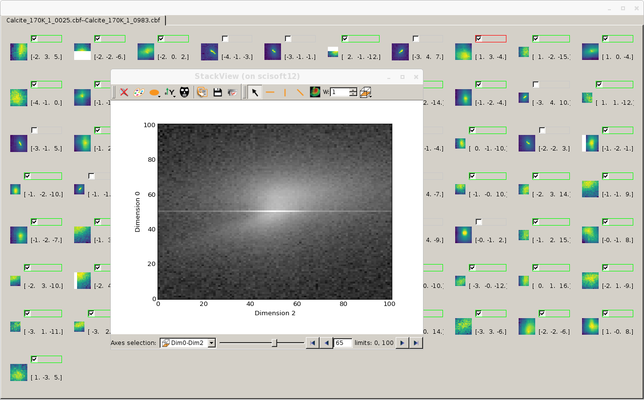
If you have set visSim=1 you can get at the end of the fit, if you are patient, back-interpolated volumes for each calculated and fitted spots. They are written in simtest.h5. To skim a compared view through selected slices of each spot
python skimma.py simetest.h5
using this script skimma.py.