Getting MgO constants out of TDS, a worked out example
Aligning the 90K dataset
This tutorial requires that you have read the documentation and worked out the Calcite example.
On the ftp site where this documentation is,
you can find first the data that you can download(17G!!!) here
MgO_data.tgz.
then the input files here
MgO_input.tgz.
Put them in the same directory and untar them. You get two subdirectories : data and analysis. In the data directory there are two subdirectories : 90 and 120 for the two different temperatures. Go now in analysis/90. Our plan is to first align and harvest at 90K, then at 120K and finally combine the two harvests in the final fit of the elastic constants.
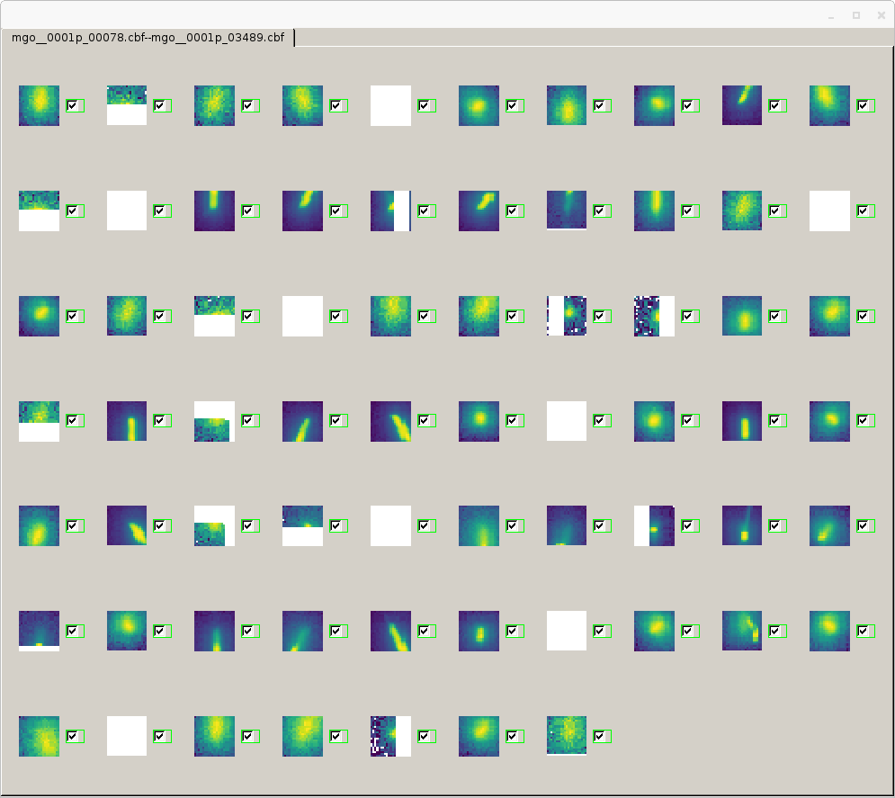
Go, in directory 90 through the sequence of first peak hunting with extraction.par. ( see calcite example for details) You get this

As you can see the Bragg reflection spots are quite large, they are the projections of the sample-beam intersection
and the sample is large ( see paper).
–For this reason in this example we will work out the geometrical alignement that will be done fitting the diffused blob–
But let us proceed as usual for now.
We are going to do a Fourier alignement on all the peaks, even those that in the screenshot appear with a blank area beacause
a peak has been detected anyway, that will be useful to get a rough peak position for preliminary alignement,
and the fine alignement will be done at TDS fitting time. To proceed run a first visualisation of your peaks
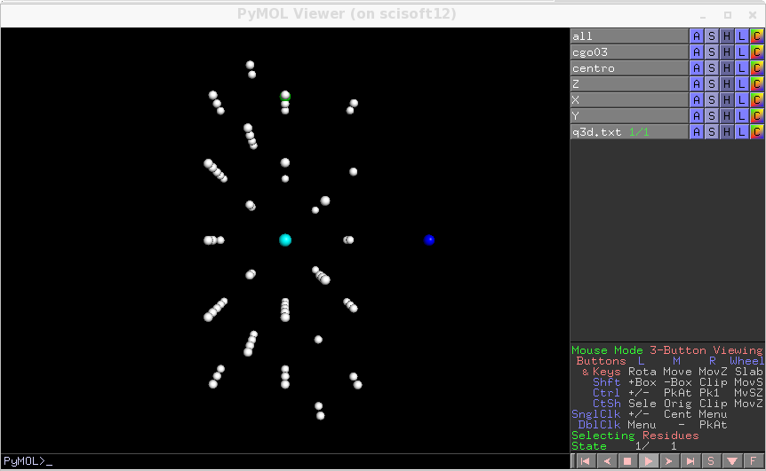
using ana0.par. to generate q3d.txt and visualise it with tds2el_rendering_vXX.
Then run tds2el_analyse_maxima_fourier_vXX ana1.par to obtain the Fourier alignement.
Notice an important point now, we have added this option in ana1.par that was not needed for Calcite
lim_aa=[4.0,4.4]
What does it mean? Several axis choices are possible, and in ana1.par we have hinted the search to search close to aAA=90,aBB=90,aCC=90 angles. But this is not enough. For MgO all the axis are commensurate and there are several possible choices to find orthogonal axes. With the lim_aa directive we ask that the first found direction for the first axis corresponds to a lattice parameter within that range ( in Angstroms). With this option you get this output
## ESTIMATION by FOURIER
AA=4.255178e+00
BB=4.255178e+00
CC=4.255178e+00
aAA=90
aBB=90   # fixed
aCC=90
r3=1.654992e+02
r2=8.877376e+01
r1=-8.946453e+01
#############
## FOLLOWING PARAMETERS ARE QUATERNIONS COEFFICIENTS.
#############
## TOBEUSED WITH USEQUAT=True
# USEQUAT=True
# r1=4.294775e-01
# r2=5.616485e-01
# r3=4.414863e-01
 ############################
- and this alignement, that you can visualise using
*ana2.par*, with transform_only option set to 1, to generate q3d.txt and the rendering script 
The output of tds2el_analyse_maxima_fourier_vXX give r1,r2,r3 in both angle and quaternionic form. This option has been added beacause in some cases, and in particular this, a particular choise of r1,r2,r3 may bring to the blocage de cardan or gimbal lock and quaternionic parameters can be used as an alternative to avoid this lock.
For a finer alignement run ana2.par with transform_only set to 0.
We have used in this ana2.par the quaternionic variables. To activate quaternionic
parameterisation USEQUAT=True and initialise r1,r2,r3 with quaternionic coefficients given by tds2el_analyse_maxima_fourier_vXX.
Notice that in ana2.par we have freed several parameters for optimisation. This is done through the variations variables.
To proceed with the fit we are going to use *tds2el_90.par* and
*tds2el_90.inp*
given in the analysis tgz file.
We need the normalisation, to get the the normalisation, always in directory analysis/90
pythonextract_norm_90_120.py
which extracts normalisation for 90K and 120K in a coherent way. The used metadata, for this experiment, is Flux which is given in each image and is an indirect measure of the intensity at the sample. This scripts generates also a file with a temperature per image. There is an option start_from that could be used, in tds2el.par, to discard the first start_from images of a scan but we are not going to use it here.
Now run tds2el_vXX first with TODO=DO_HARVESTING and using mpirun to go faster. It harvests from 0.06 to 0.15. the set TODO=FIT and rerun without mpirun, but either on a GPU host, or making use that opencl for cpu is installed and setting the devicetype ( see the doc). The provide par file is already pretty well aligned> You can add more variables, thought, to variations to align the geometry: it is fitted at the same time of elastic constants
+-------+---------------+---------------+--------------------+--------------------+--------------------+------------------+------------------+
|  A11  |      A44      |      A12      |         r1         |         r2         |         r3         |        AA        |        BB        |
+-------+---------------+---------------+--------------------+--------------------+--------------------+------------------+------------------+
| 300.0 | 194.896928547 | 30.7098674412 | -9.49498181238e-05 | -0.000174354872346 | -0.000237827707441 | 0.00197561581148 | 0.00197561581148 |
| 300.0 |      0.0      |     -400.0    |        -1.5        |        -1.5        |        -1.5        |       -0.1       |       -0.1       |
| 300.0 |     400.0     |     400.0     |        1.5         |        1.5         |        1.5         |       0.1        |       0.1        |
+-------+---------------+---------------+--------------------+--------------------+--------------------+------------------+------------------+
+------------------+------------------+-------+------+-----------------+------------------+-------------------+------------------+
|        CC        |      omega       | alpha | beta |      kappa      |        d1        |         d2        |   det_origin_X   |
+------------------+------------------+-------+------+-----------------+------------------+-------------------+------------------+
| 0.00197561581148 | 0.00698739555302 |  0.0  | 0.0  | 0.0109884853791 | 0.00658811758157 | -0.00550742840858 | 0.00941664520978 |
|       -0.1       |       -2.0       |  0.0  | 0.0  |       -2.0      |       -0.2       |        -0.2       |       -5.0       |
|       0.1        |       2.0        |  0.0  | 0.0  |       2.0       |       0.2        |        0.2        |       5.0        |
+------------------+------------------+-------+------+-----------------+------------------+-------------------+------------------+
+-------------------+
|    det_origin_Y   |
+-------------------+
| -0.00976330341494 |
|        -5.0       |
|        5.0        |
+-------------------+
 error  58528122.1314
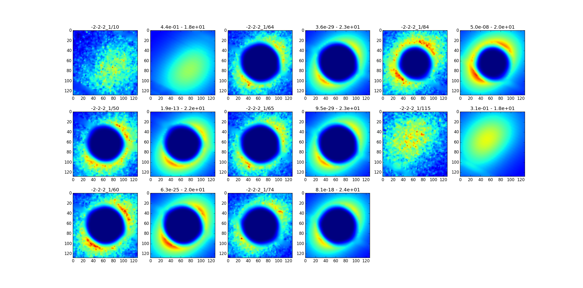
When the fit is finished the interpolation starts (visSim=1). The optimisation variables are written on parametri.txt. Except for the elastic constants, they are variations. So you must add + before = and put everything at the par file. Then if you want to do eventually a new, more centered harvesting. With the skimma.py script you can explore the fitted spots :

For the moment we skip to the 120K case to come back later on tds2el_90_bis.par.
For the harvesting we have not used the maxima_file, which could omit some weak peaks, but we have set the collectSpots variable for harvesting a small bunch of hkl plus all the replica by symmetry
REPLICA_COLLECTION = 1
For the fit we have used all the hasrvested spots : we first have done a run with show_hkls=True option, which outputs all the hkls contained in the harvesting, then we use this list to se the collectSpots variables for the fit section.
Aligning the 120K dataset
There is not much to be done for the alignement: thank to the previous work
and to the fact that the dataset was acquired moments after the 90K one,
the differences in alignement are expected to be small, so we can simply grab tds2el_90.par and tds2el_90.inp and then generate
mutata-mutandis *tds2el_120.par* and
*tds2el_120.par*.
We place them in the directory analysis/120 and we will use the analysis/90/normalisation_120.txt
and analysis/90/tagged_maxima.p already generated.
We do the usual workflow: first TODO=DO_HARVESTING then TODO=FIT, with this result
+-------+---------------+---------------+------------------+------------------+------------------+-------------------+-------------------+
|  A11  |      A44      |      A12      |        r1        |        r2        |        r3        |         AA        |         BB        |
+-------+---------------+---------------+------------------+------------------+------------------+-------------------+-------------------+
| 300.0 | 182.026073739 | 42.4839267865 | 0.00101724377872 | 0.00182279253829 | 0.00156615289279 | 0.000466549523667 | 0.000466549523667 |
| 300.0 |      0.0      |     -400.0    |       -1.5       |       -1.5       |       -1.5       |        -0.1       |        -0.1       |
| 300.0 |     400.0     |     400.0     |       1.5        |       1.5        |       1.5        |        0.1        |        0.1        |
+-------+---------------+---------------+------------------+------------------+------------------+-------------------+-------------------+
+-------------------+-----------------+-------+------+-----------------+-----------------+------------------+----------------+
|         CC        |      omega      | alpha | beta |      kappa      |        d1       |        d2        |  det_origin_X  |
+-------------------+-----------------+-------+------+-----------------+-----------------+------------------+----------------+
| 0.000466549523667 | -0.372360293271 |  0.0  | 0.0  | 0.0302214265925 | 0.0374923502485 | -0.0397007784419 | 0.042822558852 |
|        -0.1       |       -2.0      |  0.0  | 0.0  |       -2.0      |       -0.2      |       -0.2       |      -5.0      |
|        0.1        |       2.0       |  0.0  | 0.0  |       2.0       |       0.2       |       0.2        |      5.0       |
+-------------------+-----------------+-------+------+-----------------+-----------------+------------------+----------------+
+------------------+
|   det_origin_Y   |
+------------------+
| -0.0397776794745 |
|       -5.0       |
|       5.0        |
+------------------+
 error  56532761.9348
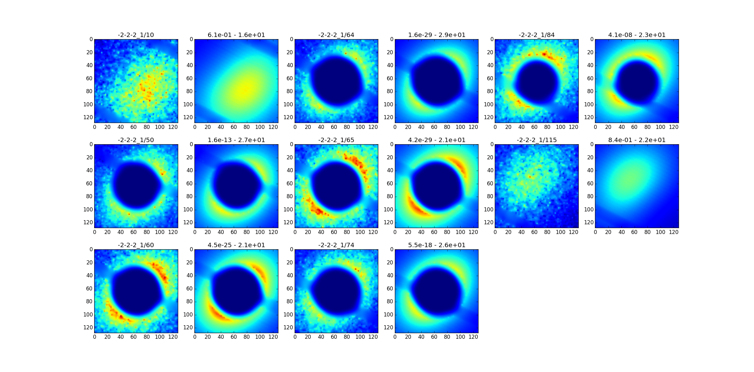
and with the skimma.py script we make sure that things look normal :

the differences in alignement are very small. We now pass to the subtraction.
Getting elastic constants by 2-temperatures subtraction
Now back to analysis/90/ directory. Both datasets are now aligned. Give this command
>tds2el_getDelta_v1 tds2el_90.par ../120/tds2el_120.par
to get this output
DELTA={
 "r1":-9.99999999973e-07,
}
the DELTA dictionary contains the differences which, added to the 90 K parameters, give the 120K ones. We create now a new input file by adding the dictionary definition at the end of tds2el_90.par to obtain and redo the harvesting on collection.h5. ( it is already done if you have used the par file as it is)
Now, thank to the DELTA option, the collected file will contain, beside the usual harvested data, additional informations that will be used to interpolate the 120K dataset to obtain interpolated datapoints that correspond to the same Q points at which we have the data points in the 90 K case.
We have now, in collection.h5 file, the interpolation informations for each data point: they are obtained calculating for each 90K data point the combination of pixels 120 K data that have to be taken in order to reproduce the same 90 K Q point using the 120 K dataset whose alignement differs by DELTA.
With this information we can clone collection.h5 using data for the 120 K dataset.
We use for this the *clone_120.inp*
input file
images_prefix         =  "../../data/120/mgo__0001p_0"
filter_file           ="../filter.edf"
file2becloned = "../90/collection.h5"
clonefile = "collection_120_cloned.h5"
normalisation_file    = "../90/normalisation_120.txt"
threshold = 1000
badradius = 0
The command is, to be given in analysis/120
tds2el_cloneinterp_v1 clone_120.inp
here images_prefix points to 120 K directory, the interpolating information is read from file2becloned,
the result goes to clonefile. The interpolation is applied on the 120 K datapoints,
after normalisation by normalisation_file.
The regions above threshold points are not used
in the fit. If badradius is zero a whole image is discarded if one of its pixels is higher that threshold.
Otherwise for each pixel above-thrshold all pixels within badradius are rejected.
Now ready for the last run.
In analysis/90 directory you find
*tds2el_MT.inp*
conf_file             =  "tds2el_MT.par"
ascii_generators      =  "2(z),2(y),3(111),2(110),1~"
DW_file="phon_e888_co900_dos.phonon.md5_code=05e9b8e2d2e2ff82f3d30660528cb1d6"
the conf_file points to the par variables where more extended variables are set, the ascii_generators is always there but probably unused, finally the DW_file is something that must have been generated with the ab2tds package and contain Debye-Waller factors for the two temperatures. This also is probably not so effective in cases where Debye-Waller factors are weak, they are used to account for the peaks intensity loss which is dependent also on temperature.
The *tds2el_MT.par*
is a simplification of tds2el_90.par, but contains links to
the two harvestings
load_from_file=[  "collection.h5",  "../120/collection_120_cloned.h5" ]
T_list        =[90, 120 ]

aAA = 90.0
aBB = 90.0
aCC = 90.0

AA = 4.2101
BB = 4.2101
CC = 4.2101

lmbda = 0.68894
# fit
nred=1
DO_ELASTIC=1

A11=269.711423956/2
A44=135.887294031*1.5
A12=105.650740784/2

CGUESS={"A11":  [A11, 0., 6000],
        "A12":  [A12, -6000, 6000],
        "A44":  [A44, -6000, 6000]
}

collectSpots = np.array(
    [[-2, -4, -2], [-2, -4, 0], [-2, -4, 2], [-2, -2, -4], [-2, -2, -2], [-2, -2, 0], [-2, -2, 2], [-2, -2, 4], [-2, 0, -4],
     [-2, 0, -2], [-2, 0, 2], [-2, 0, 4], [-2, 2, -4], [-2, 2, -2], [-2, 2, 0], [-2, 2, 2], [-2, 2, 4], [-2, 4, -2], [-2, 4, 0],
     [-2, 4, 2], [-1, -5, -1], [-1, -5, 1], [-1, -3, -3], [-1, -3, -1], [-1, -3, 1], [-1, -3, 3], [-1, -1, -5], [-1, -1, -3],
     [-1, -1, -1], [-1, -1, 1], [-1, -1, 3], [-1, -1, 5], [-1, 1, -5], [-1, 1, -3], [-1, 1, -1], [-1, 1, 1], [-1, 1, 3], [-1, 1, 5],
     [-1, 3, -3], [-1, 3, -1], [-1, 3, 1], [-1, 3, 3], [-1, 5, -1], [-1, 5, 1], [0, -4, -2], [0, -4, 0], [0, -4, 2], [0, -2, -4],
     [0, -2, -2], [0, -2, 0], [0, -2, 2], [0, -2, 4], [0, 0, -4], [0, 0, -2], [0, 0, 2], [0, 0, 4], [0, 2, -4], [0, 2, -2],
     [0, 2, 0], [0, 2, 2], [0, 2, 4], [0, 4, -2], [0, 4, 0], [0, 4, 2], [1, -5, -1], [1, -5, 1], [1, -3, -3], [1, -3, -1], [1, -3, 1],
     [1, -3, 3], [1, -1, -5], [1, -1, -3], [1, -1, -1], [1, -1, 1], [1, -1, 3], [1, -1, 5], [1, 1, -5], [1, 1, -3], [1, 1, -1], [1, 1, 1],
     [1, 1, 3], [1, 1, 5], [1, 3, -3], [1, 3, -1], [1, 3, 1], [1, 3, 3], [1, 5, -1], [1, 5, 1], [2, -4, -2], [2, -4, 0], [2, -4, 2], [2, -2, -4],
     [2, -2, -2], [2, -2, 0], [2, -2, 2], [2, -2, 4], [2, 0, -4], [2, 0, -2], [2, 0, 2], [2, 0, 4], [2, 2, -4], [2, 2, -2], [2, 2, 0], [2, 2, 2],
     [2, 2, 4], [2, 4, -2], [2,  4, 0], [2, 4, 2]]
)

doMinimisation=1
visSim=1
testSpot_beta = 0.03
testSpot_Niter = 60
testSpot_N = 128
ftol=1.e-11
density = 3.58
angular_step=0.1
here the exact values of AA,BB,CC is not so important, it is used to calculated Q at a given hkl and then the Debye-Waller strenghts at that given hkl. Now we can run the fit
>tds2elMT_v1 tds2el_MT.inp
and get
+---------------+---------------+---------------+
|      A11      |      A44      |      A12      |
+---------------+---------------+---------------+
| 319.679202141 | 160.598714478 | 95.9875135792 |
|      0.0      |    -6000.0    |    -6000.0    |
|     6000.0    |     6000.0    |     6000.0    |
+---------------+---------------+---------------+